
 , Hyung-Jin Rim1, Kwan-Dong Park1,2†, Jaewook Rhim3, Jiyeon Woo3
 1PPSOL Inc., Seoul 08504, Korea
2Department of Geoinformatic Engineering, Inha University, Incheon 22212, Korea
3Agency for Defense Development (ADD), Daejeon 34186, Korea
†Corresponding Author: Kwan-Dong Park, E-mail: kdpark@ppsol.com
Citation: Kim, Y.-G., Rim, H.-J., Park, K.-D., Rhim, J., & Woo, J. 2026, Performance Analysis of QZSS Orbit and Clock Estimation Using an Extended Kalman Filter Based on Smoothed Code Pseudorange Measurements, Journal of Positioning, Navigation, and Timing, 15, 183-194.
Journal of Positioning, Navigation, and Timing (J Position Navig Timing) 2026 June, Volume 15, Issue 2, pages 183-194. https://doi.org/10.11003/JPNT.2026.15.2.183
Received on Mar 30, 2026, Revised on Apr 14, 2026, Accepted on May 18, 2026, Published on Jun 15, 2026.
Copyright © The Institute of Positioning, Navigation, and Timing
License: Creative Commons Attribution Non-Commercial License (https://creativecommons.org/licenses/by-nc/4.0/) which permits unrestricted non-commercial use, distribution, and reproduction in any medium, provided the original work is properly cited.
GNSS, RNSS, QZSS, ODTS, SRP
A satellite navigation system enables users to determine their own position, navigation, and timing (PNT) information through broadcast navigation signals, and it is utilized as a core infrastructure in various fields such as transportation, communications, and earth science. Basically, users of a satellite navigation system perform PNT by using range measurements derived from the time difference between signal transmission at the satellite and reception by the user. To this end, users require accurate orbit and timing information from the navigation satellites. For this purpose, operators of satellite navigation systems determine the orbits and clock information of the satellites from observation data collected at global ground monitoring stations and provide this information to users (Montenbruck & Steigenberger 2020).
Today, satellite navigation systems can be classified into Global Navigation Satellite Systems (GNSS), which cover the entire globe, and Regional Navigation Satellite Systems (RNSS), which cover specific regions. Currently, the U.S. Global Positioning System (GPS), Russia’s Global Navigation Satellite System (GLONASS), and Europe’s Galileo operate as GNSS, while Japan’s Quasi‑Zenith Satellite System (QZSS) and India’s Navigation with Indian Constellation (NavIC) operate as RNSS centered on their respective countries. Meanwhile, China’s BeiDou provides global services while simultaneously offering regional services using some of its satellites.
QZSS, NavIC, and BeiDou, which began operations relatively recently, use Inclined Geosynchronous Orbit (IGSO) and Geostationary Orbit (GEO) satellites rather than the Medium Earth Orbit (MEO) satellites used by conventional GNSS. These IGSO and GEO satellites can remain over specific regions for an extended period, enabling PNT services to be provided to areas centered on their respective countries. IGSO and GEO are geosynchronous orbits; satellites in these orbits are located at an altitude of approximately 36,000 km, which is higher than that of MEO satellites at about 20,000 km. Due to their orbital characteristics, IGSO and GEO satellites require more frequent orbit maintenance maneuvers than MEO satellites (Qin et al. 2019).
In addition, when the solar elevation angle relative to the orbital plane is high, IGSO satellites in QZSS and BeiDou operate in Yaw-Steering (YS) mode, which is similar to the mode used by conventional MEO satellites. They switch to Orbit‑Normal (ON) mode when the solar elevation angle is low, whereas GEO satellites operate in ON mode at all times (Montenbruck et al. 2015a). In particular, GEO satellites have limitations in observation geometry due to their fixed positions as seen from ground observations, which fundamentally restricts their precise orbit and clock determination capabilities compared with those of MEO and IGSO satellites (Akiyama & Montenbruck 2025). Therefore, due to orbit characteristics different from those of conventional MEO satellites and limited observation conditions, the orbit determination performance of IGSO and GEO satellites is reported to remain at the level of tens of centimeters to several meters. In comparison, MEO satellites can achieve orbit determination accuracy at the centimeter level (Montenbruck et al. 2017a).
Various studies related to orbit and clock determination strategies for IGSO and GEO satellites have been conducted. Steigenberger et al. (2013) compared and analyzed the performance of various estimation strategies to identify optimal techniques for the first QZSS satellite, Michibiki-1, launched in 2010. Takasu et al. (2015), Montenbruck et al. (2017b), and Yuan et al. (2020) proposed solar radiation pressure models suitable for QZSS and evaluated orbit determination performance by comparing the results with those from existing solar radiation pressure models for navigation satellites. Additionally, Duan et al. (2019) evaluated and compared the orbit determination performance of batch processing and sequential processing techniques for navigation satellites, including the BeiDou IGSO satellite, and Roh et al. (2025) compared and analyzed the orbit and clock determination performance of QZSS satellites under QZSS alone and in combination with GPS. In summary, these studies focused on finding optimal strategies to improve the orbit and clock determination performance of IGSO and GEO satellites.
In this study, we aim to analyze the performance of orbit and clock estimation strategies that have not been thoroughly investigated in previous studies, rather than focusing on improving the estimation performance of existing IGSO/GEO satellite orbit and clock solutions or achieving centimeter-level orbit accuracy. This approach is motivated by the fact that orbit and clock estimation performance can vary depending on the estimation strategy and observation geometry, and the specific strategy adopted in this study has not been previously investigated. Orbit and clock estimation for the QZSS GEO and IGSO satellites was performed using smoothed code pseudorange measurements within an Extended Kalman Filter (EKF) framework. Without combining QZSS with other GNSS constellations, four scenarios with different numbers and combinations of QZSS satellites were designed, and the estimation performance was analyzed under identical estimation strategies. The four scenarios are classified as follows:
⋅Four QZSS satellites: three IGSO + one GEO
⋅Three QZSS satellites: two IGSO + one GEO
⋅Two QZSS satellites: one IGSO + one GEO
⋅One QZSS satellite: one IGSO
In this paper, a proprietary algorithm was developed and used to estimate the orbits and clocks of QZSS satellites. Chapter 2 provides an explanation of the estimation filters, dynamic models, and observation models constituting the developed algorithm, along with the rationale for selecting these strategies. Chapter 3 presents the analysis results for the QZSS orbit and clock estimation performance under each of the four scenarios mentioned earlier. Observation data from the International GNSS Service (IGS) reference stations (IGS 2026) were used, and the estimation performance was evaluated against the precise QZSS orbit and clock products provided by the Japan Aerospace Exploration Agency (JAXA).
The orbit and clock estimation algorithm used in this study was developed with the objective of real-time orbit and clock estimation. In general, orbit and clock determination techniques can be classified into batch and sequential processing techniques. A representative example of a batch processing technique is the ultra-rapid products produced by IGS analysis centers. According to IGS, the GPS orbit accuracy provided by ultra-rapid orbits is highly precise, on the order of about 5 cm. However, orbit predictions based on batch processing have limitations in responding to abrupt or unpredictable orbit deviations caused by unmodeled forces, orbital maneuvers, and eclipse conditions.
Lou et al. (2022) report that the ultra-rapid orbit is subject to performance degradation or even unavailability during eclipse periods or orbital maneuver intervals due to its inherent prediction-based nature. In particular, frequent orbit maintenance maneuvers of BeiDou GEO satellites are considered to adversely affect the accuracy and reliability of predicted orbits. Duan et al. (2019) evaluated the Square Root Information Filter (SRIF), one of the sequential processing techniques, and found that it provides more accurate orbits than the six-hour predicted orbits from batch processing techniques. Moreover, when the performance of the two approaches for BeiDou IGSO satellites during eclipse periods was compared, they reported that the difference in accuracy was on the order of five to six times.
The two preceding studies suggest that sequential processing techniques are more favorable than batch processing techniques for real‑time applications. However, Lou et al. (2022) noted that sequential processing techniques require robust observations and optimized stochastic models for accurate orbit and clock determination. In light of these findings, EKF was adopted as the sequential processing scheme, with careful consideration given to observation handling and filter model selection.
The EKF algorithm used in this study is based on the sequential processing algorithm proposed by Tapley et al. (2004). In general, the EKF comprises a time-update step and a measurement-update step, and the time-update is carried out using Eq. (1).
$${\overline{X}}_{i} = f\left( {\widehat{X}}_{i – 1},t_{i – 1} \right) \\
{\overline{P}}_{i} = \Phi\left( t_{i},t_{i – 1} \right){\widehat{P}}_{i – 1}\Phi^{T}\left( t_{i},t_{i – 1} \right) + Q_{i – 1}$$
where $\hat{X}_{i-1}$ and $\hat{P}_{i-1}$ denote the state vector and covariance matrix at $t_{i-1}$, respectively, while $\bar{X}_i$ and $\bar{P}_i$ denote the state vector and covariance matrix predicted to $t_i$, respectively. The notation $f$ represents the nonlinear function that propagates the state vector, $\Phi$ is the state transition matrix, and $Q$ is the covariance matrix constructed by discretizing the process noise. In this process, $\bar{X}_i$ and $\Phi(t_i,t_{i-1})$ were computed by numerically integrating the differential equations $\dot{X}$ and $\dot{\Phi}$ given in Eq. (2), and the Runge–Kutta–Fehlberg 7(8) method was used for the integration.
$$\dot{X} = F(X(t),\ t) \\
\dot{\Phi} = A(t)\Phi(t,\ t_{i – 1}),\quad A(t) = \left. \ \frac{\partial F(X,t)}{\partial X} \right|_{{\widehat{X}}_{i – 1}}$$
In Eq. (2), $F$ is a nonlinear model for the time variation of the state vector, including the satellite dynamics. The measurement-update is performed using Eq. (3).
$$y_{i} = Y_{i} – G({\overline{X}}_{i},t_{i}),\quad H_{i} = \left. \ \frac{\partial G(X,t_{i})}{\partial X} \right|_{{\overline{X}}_{i}} \\
K_{i} = {\overline{P}}_{i}{H_{i}}^{T}\left( H_{i}{\overline{P}}_{i}{H_{i}}^{T} + R_{i} \right)^{- 1} \\
{\widehat{x}}_{i} = K_{i}y_{i} \\
{\widehat{X}}_{i} = {\overline{X}}_{i} + {\widehat{x}}_{i} \\
{\widehat{P}}_{i} = \left( I – K_{i}H_{i} \right){\overline{P}}_{i}\left( I – K_{i}H_{i} \right)^{T} + K_{i}R_{i}K_{i}^{T}$$
where $y_i$ is the residual vector, $Y_i$ is the observation vector, and $G$ represents the observation model, while $H$, $K$, and $R$ denote the observation matrix, Kalman gain matrix, and observation noise covariance matrix, respectively. Finally, the state correction vector $\hat{x}$ is estimated using the Kalman gain matrix and the residual vector, and the optimal solution $\hat{X}_i$ at $t_i$ is determined accordingly. Similarly, the covariance matrix $\hat{P}_i$ is determined using the Kalman gain and the observation matrix, employing the formula proposed by Bucy & Joseph (1968) to ensure numerical stability of the filter.
The acceleration $a$ of the navigation satellite considered in this study is given by Eq. (4).
$$a = a_{geo} + a_{tide} + a_{n} + a_{rel} + a_{solar}$$
where $a_{geo}$, $a_{tide}$, $a_n$, $a_{rel}$, and $a_{solar}$ denote the accelerations due to the geopotential, tides, third-body effects, relativity, and solar radiation pressure, respectively. Among these, the accelerations due to the geopotential, tides, third‑body effects, and relativity are classified as gravitational accelerations, whereas the acceleration due to solar radiation pressure is classified as a non‑gravitational acceleration. Gravitational accelerations have the largest influence on GNSS satellite motion, but their models have already reached a high level of accuracy (Öhlinger 2022). Although the acceleration due to solar radiation pressure is smaller than gravitational accelerations, it is a major source of error in orbit determination. In particular, it significantly affects the orbit accuracy of high‑altitude satellites and is therefore treated as a key subject of research (Montenbruck et al. 2017b).
Solar radiation pressure models can generally be classified into analytical models and empirical models. A representative analytical model is the box-wing model. In the box-wing model, the satellite body is separated into the main body and solar panels, and the acceleration due to solar radiation pressure is determined based on the physical interaction between each surface and the solar radiation. The model proposed by Milani et al. (1987) is given by Eq. (5).
$$a_{solar} = – \frac{P_{sol}}{m}\sum_{i = 1}^{n}{\alpha_{i}\cos\theta_{i}\left[ 2\left( \frac{\delta_{i}}{3} + \rho_{i}\cos\theta_{i} \right){\widehat{n}}_{i} + (1 – \rho_{i})\widehat{s} \right]}$$
where $P_{sol}$ is the solar radiation pressure at 1 AU, and $m$ is the satellite mass. In addition, $n$ and $\alpha$ denote the number of surfaces in the box-wing model and each surface area, respectively. The notation $\Theta$ is the angle between the surface normal vector and the satellite–Sun vector. The vectors $\hat{n}$ and $\hat{s}$ denote the unit normal vector of the surface and the satellite–Sun unit vector, respectively, while $\delta$ and $\rho$ represent the specular reflectivity and diffusive reflectivity of the surface, respectively.
One of the most representative empirical models is the Empirical CODE Orbit Model (ECOM), developed by the Center for Orbit Determination in Europe (CODE). Unlike analytical models, ECOM (Beutler et al. 1994) describes solar radiation pressure through empirical model parameters without prior information on satellite mass, area, and other properties, and it has been mainly used for Precise Orbit Determination (POD) of GPS and GLONASS satellites (Montenbruck et al. 2015b). Although ECOM showed limitations as satellite body geometries became more complex, these issues were addressed by ECOM2 (Arnold et al. 2015). In general, the solar radiation pressure accelerations in ECOM models are defined in the orthogonal coordinate system as shown in Eq. (6).
$$e_{D} = \frac{r_{s} – r}{\left| r_{s} – r \right|},\quad e_{Y} = – \frac{e_{r} \times e_{D}}{\left| e_{r} \times e_{D} \right|},\quad e_{B} = e_{D} \times e_{Y}$$
where $r_s$ and $r$ denote the position vectors of the Sun and the satellite, respectively, and $e_r$ is the unit vector of $r$. The vector $e_D$ denotes the unit vector in the satellite–Sun direction, $e_Y$ denotes the unit vector along the solar panel axis, and $e_B$ denotes the unit vector determined by the two axes. With these axes defined, the ECOM2 model can be expressed as Eq. (7).
$$a_{solar} = a_{0} + D(u)e_{D} + Y(u)e_{Y} + B(u)e_{B} \\
D(u) = D_{0} + \sum_{i = 1}^{n_{D}}{\{ D_{2i,c}\cos 2i\mathrm{\Delta}u + D_{2i,s}\sin 2i\mathrm{\Delta}u\}} \\
Y(u) = Y_{0} \\
B(u) = B_{0} + \sum_{i = 1}^{n_{B}}{\{ B_{2i – 1,c}cos(2i – 1)\mathrm{\Delta}u + B_{2i – 1,s}sin(2i – 1)\mathrm{\Delta}u\}}$$
where $a_0$ is an optional a priori acceleration model, while $D_0$, $D_{2i,c}$, $D_{2i,s}$, $Y_0$, $B_0$, $B_{2i-1,c}$, and $B_{2i-1,s}$ denote the estimated model parameters. The values of $n_D$ and $n_B$ can be defined by the user according to the orbital characteristics, and they are generally defined using a total of nine model parameters with $n_D=2$ and $n_B=1$. The parameter $\Delta u$ is determined by the geometric relationship between the satellite and the Sun, as illustrated in Fig. 1.
Recent studies on SRP models for IGSO and GEO satellites mainly evaluate models that combine a box‑wing model with ECOM or ECOM2. The results show that using a box‑wing model combined with ECOM or ECOM2 leads to more accurate orbit and clock determination than using ECOM or ECOM2 alone (Tan et al. 2016, Montenbruck et al. 2017b, Duan et al. 2022, Yang et al. 2025). Yuan et al. (2020) found that the combined model of a five‑parameter ECOM2 and the box‑wing performs similarly to or better than the nine‑parameter ECOM2 alone. In particular, the combined model achieves comparable or higher performance with fewer model parameters than ECOM2 alone, enabling efficient orbit and clock estimation. Therefore, in this study, a model that combines the box‑wing and ECOM2 models is employed. The satellite information required for the box‑wing model is obtained from the QZSS satellite information provided by QZSS (QZSS 2026), whereas $n_D=0$ and $n_B=1$ were used for ECOM2.
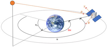
Fig. 1. Satellite–geocenter–Sun geometry, where us denotes the Sun’s argument of latitude with respect to the orbital plane.
GNSS satellite orbit and clock determination is typically based on dual-frequency code pseudoranges and carrier-phase observations. Through the ionosphere-free combination of dual-frequency measurements, most ionospheric delays can be removed, and carrier-phase observations have particularly low noise, on the order of 1–2 cm. In comparison, code pseudorange observations have noise on the order of about 1 m, and thus carrier-phase observations are employed for POD (Montenbruck & Steigenberger 2020). However, carrier-phase observations contain integer ambiguities that require a complex preprocessing procedure to resolve, which tends to extend the convergence time of orbit and clock determination. To ensure efficiency and stability in resource-constrained environments such as real-time onboard processing, Zhang et al. (2025) demonstrated the effectiveness of pseudorange-based orbit determination for IGSO satellites. Therefore, carrier-phase observations were not directly used in this study in consideration of efficiency and stability.
We used dual-frequency ionosphere-free code pseudoranges for real-time orbit and clock estimation. In addition, a carrier-phase smoothing technique based on the Hatch filter was adopted to reduce the observation noise of the raw code pseudoranges without resolving integer ambiguities (Zhang et al. 2023).
In this study, the smoothed ionosphere-free code pseudoranges are computed as follows. First, the code pseudorange and carrier-phase measurements at each frequency are given by Eq. (8).
$$P_{1} = \rho + \left( {\delta t}_{r} – {\delta t}^{s} \right) \cdot c + {\Delta I}_{1} + \mathrm{\Delta}T + \varepsilon_{P_{1}} \\
P_{2} = \rho + \left( {\delta t}_{r} – {\delta t}^{s} \right) \cdot c + {\Delta I}_{2} + \mathrm{\Delta}T + \varepsilon_{P_{2}} \\
L_{1} = \rho + \left( {\delta t}_{r} – {\delta t}^{s} \right) \cdot c – {\Delta I}_{1} + \mathrm{\Delta}T + {\lambda_{1}N}_{1} + \varepsilon_{L_{1}} \\
L_{2} = \rho + \left( {\delta t}_{r} – {\delta t}^{s} \right) \cdot c – {\Delta I}_{2} + \mathrm{\Delta}T + {\lambda_{2}N}_{2} + \varepsilon_{L_{2}}$$
where $P$ and $L$ denote the pseudorange and carrier-phase measurements expressed in meters, respectively, and the subscripts 1 and 2 indicate the corresponding frequencies. $\rho$ is the geometric distance, defined as $\rho = |r-r_r|$, with $r_r$ representing the reference station position vector. $\delta t_r$ and $\delta t^s$ denote the receiver and satellite clock errors, respectively, and $c$ is the speed of light. In addition, $\Delta I$ is the ionospheric delay, $\Delta T$ is the tropospheric delay, $\lambda$ and $N$ represent the wavelength and integer ambiguity, respectively, and is the observation noise. Frequency-specific smoothing is performed as given in Eq. (9).
$$P_{1,sm}(t_{i}) = \frac{1}{K}P_{1}(t_{i}) + \frac{K – 1}{K}[ P_{1,sm}\left( t_{i – 1} \right) + (L_{1}\left( t_{i} \right) – L_{1}\left( t_{i – 1} \right)] \\
P_{2,sm}(t_{i}) = \frac{1}{K}P_{2}(t_{i}) + \frac{K – 1}{K}[ P_{2,sm}\left( t_{i – 1} \right) + (L_{2}\left( t_{i} \right) – L_{2}\left( t_{i – 1} \right)]$$
where $P_{sm}(t_i)$ denotes the smoothed pseudorange at time $t_i$, and $K$ is the length of the Hatch filter. To apply the Hatch filter, cycle-slip detection and filter initialization are required (Hofmann-Wellenhof et al. 2008). In this study, cycle slips were detected using the Turbo-edit method proposed by Blewitt (1990), and the Hatch filter was reinitialized whenever a cycle slip was detected. The ionosphere-free combination is given by Eq. (10).
$$P_{IF,sm} = \alpha \cdot P_{1,sm} + \beta \cdot P_{2,sm},\quad \alpha = \frac{f_{1}^{2}}{f_{1}^{2} – f_{2}^{2}},\ \beta = – \frac{f_{2}^{2}}{f_{1}^{2} – f_{2}^{2}}$$
where $P_{IF,sm}$ denotes the smoothed ionosphere-free code pseudorange, and $f$ is the frequency. Finally, the observation equation of the smoothed ionosphere-free code pseudorange used for orbit and clock estimation is given by Eq. (11).
$$P_{IF,sm} = \rho + \left( {\delta t}_{r} – {\delta t}^{s} \right) \cdot c + \mathrm{\Delta}T + \varepsilon_{P_{IF,sm}}$$
In Eq. (11), $\varepsilon_{P_{IF,sm}}$ follows the observation noise model proposed by Jang et al. (2017), which is given by Eq. (12), where $T_H$ is the update interval of the Hatch filter.
$$\varepsilon_{P_{IF,sm}} = (\alpha^{2} + \beta^{2}) \cdot \varepsilon_{P_{1}}^{2} \cdot \left( \frac{T_{H}}{2K} \right)$$
In this experiment, we estimated the orbits and clocks of four QZSS satellites for three days, from 00:00:00 on 13 June 2025 to 00:00:00 on 16 June 2025 in GPS Time, using the estimation algorithm described earlier and evaluated the performance of the orbit and clock estimates. The ground network of reference stations consists of 16 IGS stations capable of receiving QZSS signals. Smoothed ionosphere‑free code pseudoranges, computed from the QZSS L1/L2 code pseudorange and carrier‑phase observations at those stations as described in Section 2.3, were used. The QZSS observation data were obtained from the Crustal Dynamics Data Information System (CDDIS), one of the IGS global data centers. The orbital type, Satellite Vehicle Number (SVN), and Pseudo Random Noise (PRN) of the QZSS satellites are listed in Table 1, and satellite ground tracks and station locations are shown in Fig. 2.
In the QZSS orbit and clock estimation experiment, the following quantities are estimated as parameters: satellite position and velocity, satellite clock error, solar radiation pressure model parameters, station clock errors, and Zenith Wet Delay (ZWD). Here, the satellite position and velocity, which are satellite‑related parameters, are estimated without considering process noise. The satellite clock error is modeled as a first‑order polynomial consisting of a bias and a drift, where both the bias and the drift are estimated as random walk processes. For each satellite, five solar radiation pressure parameters of the ECOM2 model described in Section 2.2 are estimated as random walk processes. The station clock errors, which are site‑related parameters, are estimated as biases using a random walk process, and the ZWD is estimated using a first‑order Gauss‑Markov model. All clock errors are estimated with respect to the station CCJ2 located in Japan.
The attitudes of the QZSS IGSO satellites are in YS mode by default, but switch to ON mode during orbit‑maintenance maneuvers, while the GEO satellites are always in ON mode (QZSS 2026). Since no maneuvers occurred for the IGSO satellites during the experiment period, the QZSS IGSO satellite attitudes were assumed to be in YS mode in this experiment. The observation types used are L1C(P) and L2C(L), and for stations where these observation types are not available, alternative observations at the same frequencies were used. The satellite Differential Code Bias (DCB) was corrected using products from the Deutsches Zentrum für Luft‑ und Raumfahrt (DLR), while the receiver DCB was left uncorrected. The PCO/PCV of both the satellite and ground antennas were corrected using the IGS ANTEX model (IGS 2024). The station positions were fixed to the IGS daily solutions for 13 June 2025. The tropospheric Zenith Hydrostatic Delay (ZHD) was derived from the Saastamoinen model (Saastamoinen 1972) using pressures computed by the Global Pressure Temperature (GPT) model (Boehm et al. 2007), and the ZHD values were mapped to slant hydrostatic delays using the Global Mapping Function (GMF) (Boehm et al. 2006). The initial values of the satellite position and velocity were set such that their errors relative to the precise ephemeris are within 15 km and 3 m/s, respectively, and the initial values of the SRP, satellite and receiver clock errors, and ZWD were all set to zero. The detailed conditions used for orbit and clock estimation are summarized in Table 2, and the stochastic models for each parameter in the EKF can be found in Table 3.
In orbit and clock estimation problems, a favorable spatial configuration of the observation geometry is essential to separate and estimate strongly coupled parameters. The observability of these parameters depends on the satellite–ground geometry and the spatial distribution of observations, and when this configuration is inadequate, individual parameters become difficult to estimate independently (Montenbruck & Gill 2000). Consequently, a limited observation geometry results in increased parameter correlations, which in turn degrades the accuracy of the orbit and clock estimates. Moreover, even under the same observation geometry, a significant reduction in the number of observations can considerably decrease the density of the observation data, thereby weakening the filter’s ability to separate the parameters. In consideration of these aspects, the number of satellites constituting the observation geometry was set according to the scenarios listed in Table 4, and the orbit and clock estimation performance for each case was evaluated.
The number of satellites assigned to each scenario is reduced by one satellite at a time from Scenario A to D, in descending order of SVN, regardless of the satellite orbit type, with Scenario A including all QZSS satellites operational during the experiment period. For satellites not included in a specific scenario, the satellite position and velocity, satellite clock error, and solar radiation pressure model parameters are not included in the state vector. The ground network configurations are identical in all scenarios, so the station‑based parameters, i.e., the station clock errors and ZWD, are always included in the state vector regardless of the scenario. The dynamic and observation models, as well as the stochastic models used for estimation, are kept the same across all scenarios.
The orbit and clock estimation performance was evaluated by comparing the results with the precise, final orbit and clock products from JAXA. The accuracy of the orbit estimates was assessed using the 1D, radial, along‑track, and cross‑track Root Mean Square (RMS) with respect to the precise orbit products, where the 1D is given by Eq. (13).
$$1D = \frac{3D}{\sqrt{3}} = \frac{\sqrt{{Radial}^{2} + {Along}^{2} + {Cross}^{2}}}{\sqrt{3}}$$
The estimation performance of the satellite clock errors was evaluated by first computing the difference between the bias of the estimated satellite clock error and the precise clock products, and then taking the RMS of this difference. This difference will be denoted as ‘T’ hereafter. Since the satellite clock estimates are expressed as relative values with respect to the clock error of CCJ2, they must be aligned to the same reference as the precise clock products for a valid comparison. Therefore, the estimated satellite clock error was aligned to the precise clock products according to Eq. (14).
$${\widetilde{a}}_{t_{i}}^{s} = {\widehat{a}}_{t_{i}}^{s} + a_{t_{i}}^{CCJ2} – b^{s}$$
where the superscript $s$ denotes the satellite. $\tilde{a}$ is the bias of the aligned satellite clock error, and $\hat{a}$ is the bias of the satellite clock error estimated by the filter. In addition, $a^{CCJ2}$ represents the bias of the CCJ2 clock error provided by the precise clock products, and $b$ is the satellite‑specific constant bias between the estimated satellite clock error and the precise clock products.
Table 1. QZSS Satellite orbit types, SVN, and PRN numbers.
| Orbit type | SVN | PRN |
|---|---|---|
| IGSO | J002 J004 J005 | J02 J03 J04 |
| GEO | J003 | J07 |
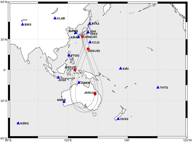
Fig. 2. QZSS satellite ground tracks and the distribution of reference stations.
Table 2. Orbit and clock estimation processing settings.
| Items | Settings |
|---|---|
Observation model Update interval Geopotential Tidal effect Third bodies Relativistic effect SRP Satellite attitude Satellite position, velocity Satellite clock error Receiver clock error Satellite DCB PCO/PCV Station position Tropospheric delay Measurement noise | Smoothed ionosphere-free pseudorange 300 sec EGM2008 8 x 8 Solid earth, ocean, pole: IERS Conventions 2010 (Petit & Luzum 2010), FES2004 Sun & Moon, All planets. Ephemeris: JPL DE440 IERS Conventions 2010 a priori box-wing model + ECOM2 5-parameter model ($n_D=0$,$n_B=1$); parameters estimated IGSO: nominal-yaw steering, GEO: orbit normal (Montenbruck et al. 2015a) Estimated as non-stochastic but time-varying parameter Estimated as bias + drift Estimated bias only DLR solution IGS ANTEX Fixed to IGS Daily solutions ZHD: GPT + Saastamoinen, ZWD: Estimated, Mapping function: GMF Elevation-dependent model and Jang et al. (2017) ($\varepsilon_{P_1}=1 m$, $K=100 sec$, $T_H=1 sec$) |
Table 3. Stochastic models for the estimated parameters.
| Parameter | Type | Process noise | Correlation time |
|---|---|---|---|
Satellite position, velocity SRP Satellite clock error Receiver clock error ZWD | Non-stochastic Random walk Random walk Random walk 1st order Gauss-Markov | – 0.005 nm/s2 Bias: 5.19×10⁻² m, Drift: 1.34×10⁻⁸ m/s Bias: Set per receiver 0.05 m | – – – – 7200 sec |
Table 4. List of satellites in each scenario.
| Scenario | # of satellites | Used SVN |
|---|---|---|
A B C D | 4 3 2 1 | J002, J003, J004, J005 J002, J003, J004 J002, J003 J002 |
The RMS values, which served as the performance metric, were computed over the time intervals during which the EKF had sufficiently converged. To define the evaluation period, the 1D and T values were plotted over time for each scenario, as shown in Fig. 3. The scenario‑wise plots are arranged in rows, with Scenarios A to D shown sequentially from top to bottom. The plot on the left of each row shows the time series of the 1D, and the plot on the right shows the time series of T. The colors in each plot indicate the SVN, and the horizontal axis represents time. For Scenarios A–C, the initial 1D and T values are on the order of tens of meters, but they gradually converge as time elapses. By contrast, in Scenario D, the 1D and T do not exhibit a clear convergence trend, and T in particular shows periodic variations nearly at the orbital period. The reason for this periodicity is explained at the end of this section. To evaluate the performance over the same time interval, the convergence interval was defined based on Scenario A. Since both the 1D and T of Scenario A show stable convergence after 48 hours, the 1D and T RMS values for all scenarios were computed for the time period after 48 hours and used as the performance metrics. The 1D, radial, along‑track, cross‑track, and T RMS values for each satellite in each scenario can be found in Fig. 4 and Table 5.
In Scenario A, the 1D RMS of the IGSO satellites J002, J004, and J005 is 3.80, 4.06, and 4.12 m, respectively, while the 1D RMS of the GEO satellite J003 is 7.43 m. In particular, the along‑track error of the GEO satellite is 12.7 m, more than twice as large as the along‑track errors of the IGSO satellites. This is attributed to the limited observation geometry of geostationary satellites, which appear fixed when viewed from the ground, and this limitation primarily degrades the along-track accuracy of GEO satellites. A similar behavior is observed in Scenarios B and C, which include GEO satellites. The T RMS, in contrast to the orbit estimation performance, shows little dependence on the orbit type, and in Scenario A the T RMS values of J002–J005 are 1.06, 1.48, 2.36, and 2.06 m, respectively. Across all scenarios, the T RMS values for each satellite are similar to the radial RMS, which is consistent with the fact that the satellite clock error is strongly coupled with the radial orbit error.
In order to simultaneously examine the changes in orbit and clock estimation performance due to the reduction in the number of satellites, the scenario‑wise mean 1D RMS and mean T RMS were computed, and the relative changes of the 1D and T RMS from Scenarios B to D, with respect to Scenario A, were evaluated. Fig. 5 shows the scenario-wise relative changes in orbit and clock estimation performance with Scenario A as the reference, and the corresponding values can be found in Table 6.
The computed mean 1D RMS values for Scenarios A to D are 4.85, 5.62, 7.08, and 21.12 m, respectively, and the mean T RMS values are 1.74, 2.02, 2.00, and 12.23 m, respectively. Overall, the orbit and clock estimation performance tends to degrade as the number of satellites decreases, and in particular, the increases in the mean 1D and T RMS in Scenario D are significantly larger than those in the other scenarios. This is because the reduction in the number of observations leads to a sharp decrease in the observability of the parameters. To explain this behavior, correlation coefficients between parameters were computed at each epoch, and the RMS of these correlation coefficients was analyzed over the performance evaluation interval. Fig. 6 shows the RMS of the correlation coefficients between the receiver clock error, which is one of the key parameters among all estimated parameters, and the orbit and clock error of the J002 satellite.
In Fig. 6, each station label denotes the receiver clock error parameter, and J002‑X, Y, Z, and T represent the three‑dimensional position and clock error parameters of the J002 satellite, respectively. Each cell in the matrix indicates the RMS of the correlation coefficient between the corresponding two parameters, with colors ranging from yellow for values close to 0 to blue for values close to 1. Therefore, a cell color closer to blue implies that the parameters are more strongly correlated and thus harder to separate. The correlations increase as the number of satellites decreases, and this trend is particularly pronounced in Scenario D. As observed in Fig. 3, the T values in Scenario D show periodic variations approximately at the orbital period. This observation implies that, in Scenario D, the correlation between the orbital components and the clock error increases significantly, resulting in degraded separability between the orbit and clock estimates. Consequently, part of the orbit error is absorbed into the clock error, leading to periodic behavior similar to the orbital period. These results demonstrate that orbit and clock estimation performance can vary significantly depending on the number of QZSS satellites used.
Table 5. RMS values of 1D, radial, along-track, cross-track, and T for each satellite under different scenarios (unit: m).
| Scenario | SVN | 1D | Radial | Along-track | Cross-track | T |
|---|---|---|---|---|---|---|
| A | J002 J003 J004 J005 | 3.80 7.43 4.06 4.12 | 1.29 1.65 2.54 1.98 | 5.43 12.7 5.38 6.09 | 3.49 1.34 3.73 3.16 | 1.06 1.48 2.36 2.06 |
| B | J002 J003 J004 | 4.35 7.88 4.64 | 1.67 1.88 2.9 | 5.75 13.4 6.43 | 4.56 1.8 3.84 | 1.57 1.73 2.77 |
| C | J002 J003 | 5.48 8.68 | 1.75 2.31 | 7.93 14.81 | 4.93 1.14 | 1.73 2.26 |
| D | J002 | 21.12 | 11.91 | 29.67 | 17.77 | 12.23 |
Table 6. Mean 1D and T RMS values and relative changes.
| Scenario | Mean 1D RMS [m] | Mean T RMS [m] | 1D change [%] | T change [%] |
|---|---|---|---|---|
A B C D | 4.85 5.62 7.08 21.12 | 1.74 2.02 2.00 12.23 | +0 +15.89 +45.90 +335.24 | +0 +16.28 +14.66 +602.87 |
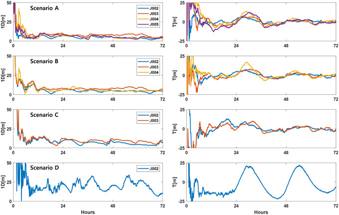
Fig. 3. Satellite-wise time series of 1D values (left four plots) and T values (right four plots) for Scenarios A–D.
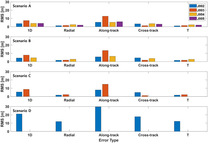
Fig. 4. Bar charts showing the 1D, radial, along-track, cross-track, and T RMS values for each satellite under different scenarios.
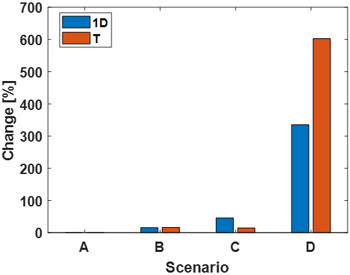
Fig. 5. Relative performance changes with respect to scenario A.
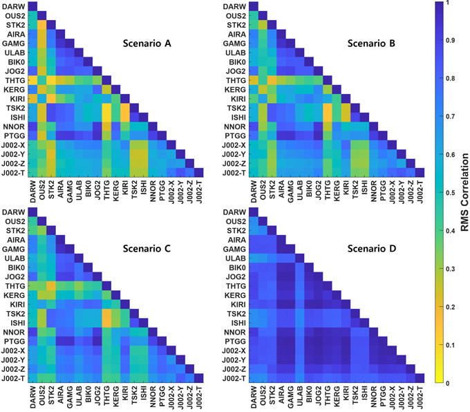
Fig. 6. RMS values of the correlation coefficients for each scenario.
In this study, we estimated the orbits and clocks of the QZSS GEO and IGSO satellites using an EKF based on smoothed code pseudoranges. The QZSS orbit and clock estimation was performed using an algorithm developed in-house, and the estimation filter, dynamic model, and observation model constituting this algorithm were described.
Using 16 IGS reference stations and the QZSS single-constellation system, the orbit and clock estimation performance of the QZSS satellites was analyzed, and the performance variation with the number of QZSS satellites included was also examined. When compared with the precise orbit and clock products from JAXA, the mean 1D RMS and mean T RMS with four QZSS satellites were 4.85 m and 1.74 m, respectively, and as the number of satellites decreased, the performance degraded to 5.62 m / 2.02 m (three satellites), 7.08 m / 2.00 m (two satellites), and 21.12 m / 12.23 m (one satellite). This degradation is interpreted as a result of increased parameter correlations with fewer satellites, and in the single‑satellite case, the observability of the parameters decreases sharply, leading to significantly lower orbit and clock estimation performance compared with the other cases.
This study quantitatively evaluated the performance of the proposed strategy for orbit and clock estimation of QZSS IGSO and GEO satellites within the QZSS single‑constellation environment, and also quantified the impact of the number of observable satellites on the orbit and clock estimation accuracy. These results are expected to provide useful guidelines for the design and operation of independent RNSSs aimed at achieving real-time, meter-level orbit and clock estimation.
This work was supported by the Agency for Defense Development by the Korean Government (UD240003TD).
Conceptualization, Y.K., H.R. and J.R.; methodology, Y.K and H. R.; software, Y.K.; validation, Y.K.; formal analysis, Y.K.; investigation, Y.K.; resources, K.P.; data curation, Y.K.; writing—original draft preparation, Y.K and K.P.; writing—review and editing, Y.K., H.R. and K.P.; visualization, Y.K.; supervision, H.R., K.P. and J.R.; project administration, Y.K.; funding acquisition, J.R. and J.W.
The authors declare no conflict of interest.
Akiyama, K. & Montenbruck, O. 2025, Along-track orbit error of geostationary GNSS satellites, Adv. Space Res., 75, 6302-6316. https://doi.org/10.1016/j.asr.2025.01.067
[DOI]
Arnold, D., Meindl, M., Beutler, G., Dach, R., & Schaer, S., et al. 2015, CODE’s new solar radiation pressure model for GNSS orbit determination, J. Geod., 89, 775-791. https://doi.org/10.1007/s00190-015-0814-4
[DOI]
Beutler, G., Brockmann, E., Gurtner, W., Hugentobler, U., Mervart, L., et al. 1994, Extended orbit modeling techniques at the CODE processing center of the international GPS service for geodynamics (IGS): theory and initial results, Manu. Geod., 19, 367-385. https://doi.org/10.1007/BF03655466
[DOI]
Blewitt, G. 1990, An automatic editing algorithm for GPS data, Geophysical Research Letters, 17, 199-202. https://doi.org/10.1029/GL017i003p00199
[DOI]
Boehm, J., Niell, A., Tregoning, P., & Schuh, H. 2006, Global Mapping Function (GMF): A new empirical mapping function based on numerical weather model data, Geophysical Research Letters, 33, L07304. https://doi.org/10.1029/2005GL025546
[DOI]
Boehm, J., Heinkelmann, R., & Schuh, H. 2007, Short note: A global model of pressure and temperature for geodetic applications, Journal of Geodesy, 81, 679-683. https://doi.org/10.1007/s00190-007-0132-5
[DOI]
Bucy, R. S. & Joseph, P. D. 1968, Filtering for Stochastic Processes with Applications to Guidance (New York: Interscience Publishers).
Duan, B., Hugentobler, U., Chen, J., Selmke, I., & Wang, J. 2019, Prediction versus real-time orbit determination for GNSS satellites, GPS Solut., 23, 39. https://doi.org/10.1007/s10291-019-0834-2
[DOI]
Duan, B., Hugentobler, U., Selmke, I., Marz, S., Killian, M., et al. 2022, BeiDou Satellite Radiation Force Models for Precise Orbit Determination and Geodetic Applications, IEEE Transactions on Aerospace and Electronic Systems, 58, 2823-2836. https://doi.org/10.1109/TAES.2021.3140018
[DOI]
Hofmann-Wellenhof, B., Lichtenegger, H., & Wasle, E. 2008, GNSS – Global Navigation Satellite Systems: GPS, GLONASS, Galileo, and more (Wien/New York: Springer)
IGS 2024, IGS Antenna Working Group [Internet], cited 2026 Mar 26, available from: https://igs.org/wg/antenna/
IGS 2026, IGS network [Internet], cited 2026 Mar 26, available from: https://network.igs.org/
Jang, J., So, H., Lee, K., & Park, J.‑P. 2017, A theoretical and experimental comparison of the ionosphere‑free L1 pseudorange and the ionosphere‑free linear combination pseudorange by dual‑frequency SBAS users, IET Radar, Sonar and Navigation, 11, 675‑681. https://doi.org/10.1049/iet‑rsn.2016.0397
[DOI]
Lou, Y., Dai, X., Gong, X., Li, C., Qing, Y., et al. 2022, A review of real-time multi-GNSS precise orbit determination based on the filter method, Satellite Navigation, 3, 15. https://doi.org/10.1186/s43020-022-00075-1
[DOI]
Milani, A., Nobili, A. M., & Farinella, P. 1987, Non-gravitational Perturbations and Satellite Geodesy (Bristol: Adam Hilger).
Montenbruck, O. & Gill, E. 2000, Satellite Orbits: Models, Methods and Applications (Berlin/Heidelberg: Springer).
[DOI]
Montenbruck, O., Schmid, R., Mercier, F., Steigenberger, P., Noll, C., et al. 2015a, GNSS Satellite Geometry and Attitude Models, Adv. Space Res., 56, 1015-1029. https://doi.org/10.1016/j.asr.2015.06.019
[DOI]
Montenbruck, O., Steigenberger, P., & Hugentobler, U. 2015b, Enhanced solar radiation pressure modeling for Galileo satellites, J. Geod., 89, 283-297. https://doi.org/10.1007/s00190-014-0774-0
[DOI]
Montenbruck, O., Steigenberger, P., Prange, L., Deng, Z., Zhao, Q., et al. 2017a, The Multi-GNSS Experiment (MGEX) of the International GNSS Service (IGS) – Achievements, prospects and challenges, Advances in Space Research, 59, 1671-1697. https://doi.org/10.1016/j.asr.2017.01.011
[DOI]
Montenbruck, O., Steigenberger, P., & Darugna, F. 2017b, Semi-analytical solar radiation pressure modeling for QZS-1 orbit-normal and yaw-steering attitude, Adv. Space Res., 59, 2088-2100. https://doi.org/10.1016/j.asr.2017.01.036
[DOI]
Montenbruck, O. & Steigenberger, P. 2020, GNSS Orbit Determination and Time Synchronization, in Position, Navigation, and Timing Technologies in the 21st Century, eds. Morton, Y. T. J., van Diggelen, F., Spilker Jr., J. J., Parkinson, B. W., Lo, S., et al. (Hoboken: John Wiley & Sons). https://doi.org/10.1002/9781119458449.ch11
[DOI]
Öhlinger, F. L. 2022, Precise orbit determination of BeiDou satellites focusing on solar radiation pressure models, Master’s Thesis, Graz University of Technology.
Petit, G. & Luzum, B. 2010, IERS Conventions (2010), IERS Conventions Centre, IERS Technical Note No.36.
Qin, Z., Huang, G., Zhang, Q., Wang, L., Yan, X., et al. 2019, Precise Orbit Determination for BeiDou GEO/IGSO Satellites during Orbit Maneuvering with Pseudo-Stochastic Pulses, Remote Sensing, 11, 2587. https://doi.org/10.3390/rs11212587
[DOI]
QZSS 2026, QZSS Satellite Information [Internet], cited 2026 Mar 26, available from: https://qzss.go.jp/en/technical/qzssinfo/index.html
Roh, K.-M., Kim, G., & Park, E. 2025, Investigating Ground Station Deployment Strategies to Improve Quality of Orbit Determination of Regional Navigation Satellite System, JPNT, 14, 353-363. https://doi.org/10.11003/JPNT.2025.14.4.353
[DOI]
Saastamoinen, J. 1972, Contributions to the theory of atmospheric refraction, Bulletin Géodésique, 105, 279‑298. https://doi.org/10.1007/BF02521844
[DOI]
Steigenberger, P., Hauschild, A., Montenbruck, O., Rodriguez-Solano, C., & Hugentobler, U. 2013, Orbit and Clock Determination of QZS-1 Based on the CONGO Network, Navigation, 60, 31-40. https://doi.org/10.1002/navi.27
[DOI]
Takasu, T., Miyoshi, M., Kawate, K., & Kogure, S. 2015, QZSS-1 Precise Orbit Determination by MADOCA, in Proceedings of the International Symposium on GNSS 2015, Kyoto, Japan, 16-18 November 2015.
Tapley, B. D., Schutz, B. E., & Born, G. H. 2004, Statistical Orbit Determination (San Diego: Elsevier Science).
[DOI]
Tan, B., Yuan, Y., Zhang, B., Hsu, H. Z., & Ou, J. 2016, A new analytical solar radiation pressure model for current BeiDou satellites: IGGBSPM, Sci. Rep., 6, 32967. https://doi.org/10.1038/srep32967
[DOI]
Yang, C., Guo, J., Xu, X., Wang, L., & Zhao, Q. 2025, Solar radiation pressure models for BDS-3 IGSO: Impacts and improvement from observation geometry, Measurement Science and Technology, 36, 036308. https://doi.org/10.1088/1361-6501/ad9e0c
[DOI]
Yuan, Y., Li, X., Zhu, Y., Xiong, Y., Huang, J., et al. 2020, Improving QZSS precise orbit determination by considering the solar radiation pressure of the L-band antenna, GPS Solut., 24, 50. https://doi.org/10.1007/s10291-020-0963-7
[DOI]
Zhang, Q., Ma, X., Gao, Y., Huang, G., & Zhao, Q. 2023, An improved carrier‑smoothing code algorithm for BDS satellites with SICB, Remote Sensing, 15, 5253. https://doi.org/10.3390/rs15215253
[DOI]
Zhang, Z., Huang, Y., Yang, P., Chen, Y., & Jia, X. 2025, Orbit determination analysis of IGSO satellite onboard GPS/BDS pseudorange data corrected by different code hardware delays products, Advances in Space Research, 75, 3050‑3062. https://doi.org/10.1016/j.asr.2024.11.047
[DOI]